Tutorial 6: Future regressors#
To model future regressors, both past and future values of these regressors have to be known. So in contrast to the lagged regressors in the previous tutorial, future regressors also have a forecasted value for the future in addition to the historic values.
[1]:
import pandas as pd
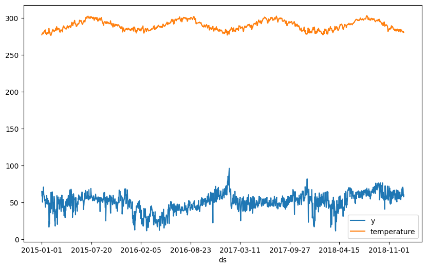
# Load the dataset for tutorial 4 with the extra temperature column
df = pd.read_csv("https://github.com/ourownstory/neuralprophet-data/raw/main/kaggle-energy/datasets/tutorial04.csv")
df.head()
[1]:
| ds | y | temperature | |
|---|---|---|---|
| 0 | 2015-01-01 | 64.92 | 277.00 |
| 1 | 2015-01-02 | 58.46 | 277.95 |
| 2 | 2015-01-03 | 63.35 | 278.83 |
| 3 | 2015-01-04 | 50.54 | 279.64 |
| 4 | 2015-01-05 | 64.89 | 279.05 |
[2]:
fig = df.plot(x="ds", y=["y", "temperature"], figsize=(10, 6))
[3]:
from neuralprophet import NeuralProphet, set_log_level

# Disable logging messages unless there is an error
set_log_level("ERROR")

# Model and prediction
m = NeuralProphet(
    n_changepoints=10,
    yearly_seasonality=True,
    weekly_seasonality=True,
    daily_seasonality=True,
    n_lags=10,
)
m.set_plotting_backend("plotly-static")

# Add the new future regressor
m.add_future_regressor("temperature")

# Continue training the model and making a prediction
metrics = m.fit(df)
forecast = m.predict(df)
m.plot(forecast)

[4]:
m.plot_components(forecast, components=["future_regressors"])

[5]:
m.plot_parameters(components=["future_regressors"])

[6]:
metrics
[6]:
| MAE | RMSE | Loss | RegLoss | epoch | |
|---|---|---|---|---|---|
| 0 | 67.432861 | 79.714500 | 0.789800 | 0.0 | 0 |
| 1 | 40.313995 | 49.790257 | 0.434656 | 0.0 | 1 |
| 2 | 23.730885 | 29.712715 | 0.221153 | 0.0 | 2 |
| 3 | 13.360303 | 17.117233 | 0.094893 | 0.0 | 3 |
| 4 | 10.110947 | 13.336704 | 0.061117 | 0.0 | 4 |
| ... | ... | ... | ... | ... | ... |
| 95 | 4.837646 | 6.482005 | 0.016463 | 0.0 | 95 |
| 96 | 4.830614 | 6.461479 | 0.016331 | 0.0 | 96 |
| 97 | 4.829221 | 6.457165 | 0.016324 | 0.0 | 97 |
| 98 | 4.823629 | 6.465248 | 0.016352 | 0.0 | 98 |
| 99 | 4.838150 | 6.507308 | 0.016487 | 0.0 | 99 |
100 rows × 5 columns
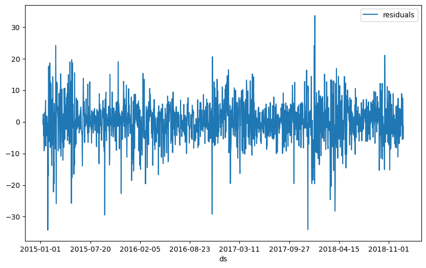
[7]:
df_residuals = pd.DataFrame({"ds": df["ds"], "residuals": df["y"] - forecast["yhat1"]})
fig = df_residuals.plot(x="ds", y="residuals", figsize=(10, 6))