Tutorial 5: Lagged regressors

Lagged regressors are used to correlate other observed variables to our target time series. For example the temperature of the previous days might be a good predictor of the temperature of the next day.

They are often referred to as exogenous variables or as covariates. Unlike future regressors, the future of a lagged regressor is unknown to us.

At the time \(t\) of forecasting, we only have access to their observed, past values up to and including \(t − 1\).

\[\text{Lagged regressor}(t) = L(t) = \sum_{x \in X}L_x(x_{t-1},x_{t-2},...,x_{t-p})\]

First we load a new dataset which also contains the temperature.

import pandas as pd

# Load the dataset for tutorial 4 with the extra temperature column
df = pd.read_csv("https://github.com/ourownstory/neuralprophet-data/raw/main/kaggle-energy/datasets/tutorial04.csv")
df.head()

	ds	y	temperature
0	2015-01-01	64.92	277.00
1	2015-01-02	58.46	277.95
2	2015-01-03	63.35	278.83
3	2015-01-04	50.54	279.64
4	2015-01-05	64.89	279.05

# Optional:To align the scale of temperature with the energy price, we convert it to Farenheit:
df["temperature"] = (df["temperature"] - 273.15) * 1.8 + 32

fig = df.plot(x="ds", y=["y", "temperature"], figsize=(10, 6))

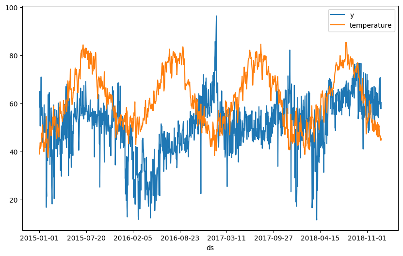
From the data we can see that there is a weak inverse relationship of electricity price to temperature. We start with our model from the previous tutorial and then add temperature as a lagged regressor to our model.

from neuralprophet import NeuralProphet, set_log_level

# Disable logging messages unless there is an error
set_log_level("ERROR")

# Model and prediction
m = NeuralProphet(
    n_changepoints=10,
    yearly_seasonality=True,
    weekly_seasonality=True,
    daily_seasonality=False,
    n_lags=10,  # Autogression
)
m.set_plotting_backend("plotly-static")

# Add temperature of last three days as lagged regressor
m.add_lagged_regressor("temperature", n_lags=3)

# Continue training the model and making a prediction
metrics = m.fit(df)
forecast = m.predict(df)

# set plotting to focus on forecasting horizon 1 (the only one for us here)
m.highlight_nth_step_ahead_of_each_forecast(1)
m.plot(forecast)

# show the component's forecast contribution
m.plot_components(forecast, components=["lagged_regressors"])

We see that the temperatur impact the forecasted price by few units. Compared to the overall price fluctuations, the temperature impact seems minor, but not insignificant.

# visualize model parameters of lagged regression
m.plot_parameters(components=["lagged_regressors"])

The model learns a different weights for each of the lags, which may also capture changes in the direction of temperature.

Let us explore how our model improved after adding the lagged regressor.

metrics.tail(1)

	MAE	RMSE	Loss	RegLoss	epoch
172	4.936666	6.578746	0.00533	0.0	172

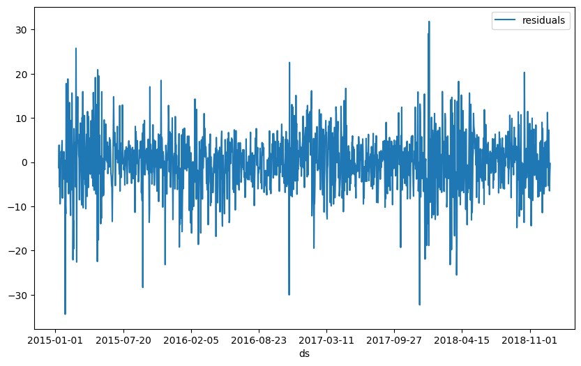
df_residuals = pd.DataFrame({"ds": df["ds"], "residuals": df["y"] - forecast["yhat1"]})
fig = df_residuals.plot(x="ds", y="residuals", figsize=(10, 6))